Week 7: Binning genomes with anvi’o
Intro (Rika will go over this at the beginning of lab)
This week in lab we’ll learn how disentangle individual microbial genomes from your mess of metagenomic contigs. We aren’t going to use a toy dataset this week—-we’re going straight into analysis with your metagenome datasets for your projects.
Genomes are disentangled from metagenomes by clustering contigs according to two properties: coverage and tetranucleotide frequency. Basically, if contigs have similar coverage patterns between datasets, they are clustered together; and if contigs have similar kmers, they will cluster together. When we cluster contigs together like this, we get a collection of contigs that are thought to represent a reconstruction of a genome from your metagenomic sample. We call these ‘genome bins,’ or ‘metagenome-asembled genomes’ (MAGs). We will talk more about this in class.
There is a lot of discussion in the field about which software packages are the best for making these genome bins. And of course, the one you choose will depend a lot on your dataset, what you’re trying to accomplish, and personal preference. I chose anvi’o because it is a nice visualization tool that builds in many handy features.
I am drawing a lot of information for this tutorial from the anvi’o website. If you’d like to learn more, see this link.
Getting your contigs ready for anvi’o
1. ssh tunnel
As always, boot onto the Mac OS and open up your Terminal application. But don’t ssh the normal way! Anvio requires visualization through the server, so this week we have to create what is called an “ssh tunnel” to log into the server in a specific way. Substitute “username” below with your own Carleton login name.
NOTE: Each of you will be assigned a different port number (i.e. 8080, 8081, 8082, etc.). I’ll put that on the white board. Substitute your assigned port number for 8080 shown below.
ssh -L 8080:localhost:8080 username@baross.its.carleton.edu
2. Make new folder
Make a new directory called “anvio” inside your project folder, then change into that directory.
cd project_directory
mkdir anvio
cd anvio
3. Copying the co-assembly
In previous weeks, you’ve been working with assembled contigs of your own samples. This week, we’ll be working with a co-assembly of all of the Tara samples assembled together. This tends to produce better bins.
Not only that, I’ve done some Martha Stewart-style pre-baking for you and I have made a contigs database out of this co-assembly, ready for use by anvi’o. Basically, I put the co-assembled contigs as well as information from Prokka about ORFs and annotations all into a single database. It is conveniently called contigs.db. (If you want more information about how I did this, visit the anvi’o tutorial I linked above.)
To copy the co-assembly database into your own folder, do this:
cp /workspace/data/Genomics_Bioinformatics_shared/anvio_stuff/contigs.db .
4. Copying the BAM files
Remember that bins are made from information based on tetranucleotide frequencies and coverage. The contigs database I made for you contains information about tetranucleotide frequencies. To get coverage information, we need to use BAM files based on mappings of reads to the co-assembly. Fortunately for you, I have already mapped all of the Tara metagenomes against the co-assembled contigs. I have also created “Profiles” of those BAM files, which formats them in a way used by anvi’o. (Again, if you want more information about how I did this, see the anvi’o tutorial above.)
They are in this folder:
/workspace/data/Genomics_Bioinformatics_shared/anvio_stuff/mapped_files
Copy up to six anvi’o profiles from that folder, depending on which samples you’re interested in. You have to copy recursively (cp -r) because they’re folders, not files.
For example:
cp -r /workspace/data/Genomics_Bioinformatics_shared/anvio_stuff/mapped_files/mega_assembly_minlength2500_vs_ERR599104_sorted.bam-ANVIO_PROFILE/ .
cp -r /workspace/data/Genomics_Bioinformatics_shared/anvio_stuff/mapped_files/mega_assembly_minlength2500_vs_ERR599090_sorted.bam-ANVIO_PROFILE/ .
cp -r /workspace/data/Genomics_Bioinformatics_shared/anvio_stuff/mapped_files/mega_assembly_minlength2500_vs_ERR599008_sorted.bam-ANVIO_PROFILE/ .
5. Merge them together with anvi-merge
Now we have to merge all of these profiles together using a program called anvi-merge. See below.
The asterisk * is a wildcard that tells the computer, ‘take all of the folders called ‘PROFILE.db’ from all of the directories and merge them together.’
If you have a sample with tons of contigs, this command may decide not to cluster your contigs together. We’re going to force it to do that with the --enforce-hierarchical-clustering flag.
This step will take a couple minutes.
anvi-merge */PROFILE.db -o SAMPLES-MERGED -c contigs.db --enforce-hierarchical-clustering
Visualizing and making your bins
6. anvi-interactive
Now the fun part with pretty pictures! Type this to open up the visualization of your contigs (of course, change the port number to the one you were assigned):
anvi-interactive -p SAMPLES-MERGED/PROFILE.db -c contigs.db -P 8080
7. Visualize in browser
Now, open up a browser (Chrome works well) and type this into the browser window to stream the results directly from the server to your browser. Use the port number (i.e. 8080, 8081, 8082, etc) that you logged in with in the first step.
http://localhost:8080
Cool, eh?
Click ‘Draw’ to see your results! You should see something like this:
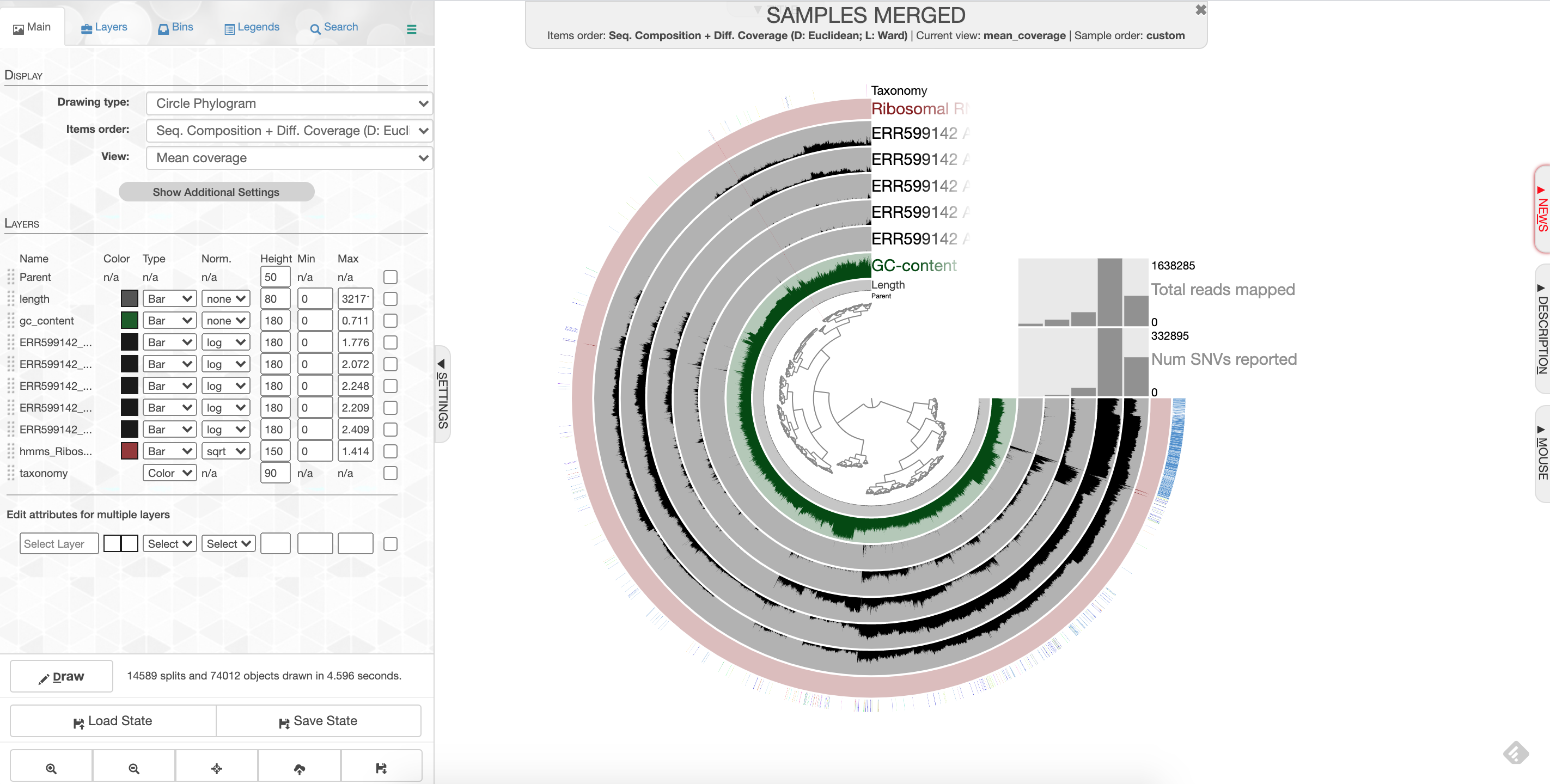 anvio screenshot
What you are looking at:
- the tree on the inside shows the clustering of your contigs. Contigs that were more similar according to k-mer frequency and coverage clustered together.
- the rings on the outside show your samples. Each ring is a different sample. This is a visualization of the mapping that you did last week, but now we can see the mapping across the whole sample, and for all samples at once. There is one black line per contig. The taller the black line, the more mapping for that contig.
- the ‘ribosomal proteins’ ring shows contigs with hits to known ribosomal proteins (useful for some applications)
- the ‘taxonomy’ ring shows the Centrifuge designation for the taxonomy of that particular contig.
- the ‘GC content’ ring shows the average percent of bases that were G or C as opposed to A or T for that contig.
8. Make bins
We will go over the process for making bins together in class.
Because your datasets are fairly small, your bins are also going to be very small. Your percent completeness will be very low. Try to identify ~3-5 bins according to patterns in the mapping of the datasets as well as the GC content.
When you are done making your bins, be sure to click on ‘Store bin collection’, give it a name (’my_bins’ works), and then click on ‘Generate a static summary page,’ click on the name of your bin collection (e.g. “my_bins”), and then click on the link it gives you. It will provide lots of information about your bins. In the boxes under the heading ‘taxonomy,’ you can click on the box to get a percentage rundown of how many contigs in your bin matched specific taxa according to centrifuge, if any matched.
Once you have completed your binning process, take a screenshot of your anvi’o visualization and save it as ‘Figure 1.’ Write a figure caption explaining what your project dataset is, and which datasets you mapped to your sample.
9. Finding bin information
You will find your new bin FASTA files in the directory called ~/project_directory/anvio/SAMPLES-MERGED/SUMMARY_my_bins. I’ll describe all this information below for reference; it may come in handy if you decide to use this for your final project.
bins_summary.txtprovides just that, with information about the taxonomy, total length, number of contigs, N50, GC content, percent complete, and percent redundancy of each of your bins. This is reflected in the summary html page you generated earlier when you clicked ‘Generate a static summary page.’
If you go to the directory bins_across_samples, you will find information about all of your bins across all samples, such as:
mean_coverage.txt, which gives the average coverage of your bins across all samplesvariability.txt, which gives you the number of single nucleotide variants (SNVs) per bin in each sample
If you want to know what the rest of these files mean, look here.
If you go to the directory bin_by_bin, you will find a series of directories, one for each bin you made. Inside each directory is a wealth of information about each bin. This includes (among other things):
- a FASTA file containing all of the contigs that comprise your bin (i.e.
Bin_1-contigs.fa) - a file with all of the gene sequences and gene annotations in your bin (i.e.
Bin_1-gene-calls.txt) - mean coverage of your bin across all of your samples (i.e.
Bin_1-mean-coverage.txt) - files containing copies of single-copy, universal genes found in your contigs (i.e.
Bin_1-Archaea-76-hmm-sequences.txtandBin_1-Bacteria_71-hmm-sequences.txt - information about single nucleotide variability in your bin– the number of SNVs per kilobase pair. (i.e.
Bin_1-variability.txt)
10. Estimating the metabolism of these genomes
One of the most powerful things about bins is that we can look inside these genomes, see their taxonomy (i.e. who they are), and try to guess what metabolisms they have (i.e. what functions are they performing in the habitat). anvi’o can help us use our Prokka annotations to estimate the metabolism of your bins. We will use anvi-estimate-metabolism to do this.
Type this:
anvi-estimate-metabolism -c contigs.db -p SAMPLES-MERGED/PROFILE.db -C my_bins --kegg-data-dir /workspace/data/Space_Hogs_shared_workspace/databases/anvio_kegg_database
-clists your contigs database, which has the Prokka information to identify metabolic genes-plists your BAM files in the PROFILE folders, which can tell you the coverage of these metabolic genes-Cgives information about the bins you choose--kegg-data-dirgives directions to the whole KEGG database, which I downloaded earlier for you, to help categorize these genes using the KEGG database
Analyzing your bins
All right! You now have an output file called kegg-metabolism-modules.txt. I recommend that you use scp to download this to your computer, and take a look at it in Excel.
Here’s what the columns mean:
bin_name: the bin name that anvi’o assigned your bins as you were making them, i.e. “Bin_1.”kegg_module: the pathway that the gene can be found in, as assigned by KEGG. See here for more information.module_name: the name of the KEGG module in which the gene is foundmodule_class: the type of module it’s found in. It can be a “pathway module,” or a gene in a metabolic pathway, a “signature module”, or a gene that characterizes a specific phenotype like drug resistance or pathogenicity, or a “reaction module,” a set of genes that catalyze successive reactions (these are usually extensions of specific metabolic pathways.)module category: is the broadest category in which the metabolic pathway is found, i.e. “Carbohydrate metabolism”module subcategory: one level down in terms of categories in which the metabolic pathway is found, i.e. “Carbon fixation”module definition: the list of genes that are found in a pathway or module, listed by their KO (or “KEGG Orthology”) number, which is how KEGG labels different genesmodule completion: how complete the pathway is. If your metabolic pathway has 10 genes in it, and 6 of them are present in your bin, this value will be 0.6.module_is_complete: this will only say ‘TRUE’ if your module completion value is 75% or above.kofam_hits_in_module: tells you exactly which genes from the pathway were present in your bingene_caller_ids_in_module: tells you which gene numbers from Prokka (and re-numbered by anvi’o) were in your pathway.
Postlab assignment
For this week’s postlab assignment, there are a few “check for understanding” questions and a mini research question.
A. Check for understanding
- In the anvi’o visualization, what does each of the “leaves” of the tree represent? What is the clustering meant to indicate (i.e. what do the branches on the tree represent)?
- In the anvi’o visualization, what does each of the grey rings represent? Which file contained the data needed to create each of those rings?
- Everyone in the class was working with the same co-assembly, and yet the clustering of the contigs in the anvi’o wheel might have looked different between different people in the class. Using what you know about how bins are made, explain why this might be the case.
B. Mini research question
Use your anvi’o outputs to do some data exploration to ask and answer a scientific question. I’d recommend paying the most attention to two output files: kegg-metabolism-modules.txt and SAMPLES-MERGED/SUMMARY_my_bins/bins_across_samples/mean_coverage.txt, but you’re welcome to use any of the anvi’o output you like.
Turn in Figure 1 with a figure caption, the three “check for understanding” questions, and your mini research question in by lab next week on the class Moodle page.